Understanding Gabor Filter

This is an informal tutorial on the intuitive theory behind gabor filters used for image segmantation.

Objective:

We formulate the intuitive theory behind making a gabor filters from first principles. All the detailed derivation of the formulae is laid out in the appendix, so if you just want to take these formulae as granted, a firm grasp in fourier transforms is not essential. We also try out the results of these formulae and plot them in octave.

Notation:

The following notation is used in this post.

$$\begin{eqnarray*} h(t) & = & \text{one dimensional gaussian function} \\ \mathscr{F}(p(t)) & = & P(f) \space \text{,fourier transform of function} \space p(t) \\ h(x,y) & = & \text{two dimensional gaussian function} \\ \mathscr{F}(p(x, y)) & = & P(u, v) \space \text{,fourier transform of 2D function} \space p(x, y) \\ H(u, v) & = & \mathscr{F}(h(x, y)) \space \text{fourier transform of 2D gaussian} \\ g(x,y) & = & \text{complex 2D gabor function (in various forms)} \\ G(u, v) & = & \mathscr{F}(g(x, y)) \\ \text{exp}(t) & = & \text{same as } \space e^{t} \end{eqnarray*}$$

Formulate the formulae for gabor filter

Gaussian function and its fourier transform

The equation for a one dimensional gaussian function is

$$\begin{equation} \label{eqa} h(t) = \frac{1}{\sqrt{2\pi}\sigma}e^{-\frac{t^2}{2\sigma^2}} \end{equation}$$

For a general function $p(t)$, the fourier transform $\mathscr{F}(p(t)) = P(f)$ is given by,

$$\begin{equation} \label{eqv} P(f) = \int_{-\infty}^{\infty} p(t) e^{-i2\pi f t} dt \end{equation}$$

From \eqref{eqf}, fourier transform $\mathscr{F}(h(t)) = H(f)$ of $h(t)$ in \eqref{eqa} is,

$$\begin{eqnarray} \label{equ} H(f) & = & \frac{1}{\sqrt{2\pi}\sigma} \sqrt{2\pi}\sigma e^{-2\pi^2f^2\sigma^2} \\ & = & e^{-2\pi^2f^2\sigma^2} \\ \end{eqnarray}$$

Introducing one dimensional gabor filter

Consider the functions $g_{e}(t) = h(t) cos(2 \pi f_1 t)$ and $g_{o}(t) = h(t) sin(2 \pi f_1 t)$, which are gaussian functions modulated by a cosine and a sine function respectively, where $f_1$ is a fixed frequency.

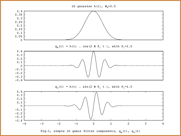
The plots of the functions $h(t), g_e(t)$ and $g_o(t)$ are shown above.

The one dimensional complex gabor filter is given by

$$\begin{eqnarray} \label{eqq} g(t) & = & g_e(t) + i g_o(t) \\ & = & h(t) ( cos(2 \pi f_1 t) + i sin(2 \pi f_1 t))\\ & = & h(t) e^{i2\pi f_1} \end{eqnarray}$$

Please note that the fourier transform of the product of two functions, $p(t)$, $q(t)$, is the convolution of their respective fourier transforms, ie $P(f) * Q(f)$.

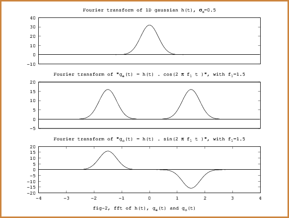
Let us do a fourier analysis of $g_{e}(t)$ and $g_{o}(t)$.

$$\begin{eqnarray} \label{eqn} \mathscr{F}(g_e(t)) & = & G_{e}(f) & = & H(f) * C(f)\\ \mathscr{F}(g_e(t)) & = & G_{o}(f) & = & H(f) * S(f) \end{eqnarray}$$

Since $p(x) * q(x) = \int_{-\infty}^{\infty} p(t) q(x - t) dt$ and since convolution is commutative, and using \eqref{eql}, \eqref{eqf},

$$\begin{eqnarray} \label{eqo} G_{e}(f) & = & \int_{-\infty}^{\infty} C(u) H(f - u) du \\ & = & \frac{1}{2} \int_{-\infty}^{\infty} H(f - u) (\delta(u + f_1) + \delta(u - f_1)) du\\ & = & \frac{1}{2} ( H(f + f_1) + H(f - f_1) ) \\ & = & \frac{1}{2} ( e^{-2\pi^2(f + f_1)^2\sigma^2} + e^{-2\pi^2(f - f_1)^2\sigma^2} ) \end{eqnarray}$$

So by \eqref{eqq}, the real part of the fourier transform of $g_e(t)$ is the sum of two gaussian functions separated by $\pm f_1$, and the imaginary part is the difference of two gaussian finctions separeted by $\pm f1$.

Similarly, $\begin{eqnarray} \label{eqp} G_{o}(f) & = & \int_{-\infty}^{\infty} S(u) H(f - u) du \\ & = & \frac{i}{2} \int_{-\infty}^{\infty} H(f - u) (\delta(u + f_1) - \delta(u - f_1)) du\\ & = & \frac{i}{2} ( H(f + f_1) - H(f - f_1) ) \\ & = & \frac{i}{2} ( e^{-2\pi^2(f + f_1)^2\sigma^2} - e^{-2\pi^2(f - f_1)^2\sigma^2} ) \end{eqnarray}$

Similarly, $\begin{eqnarray} \label{eqp2} G(f) & = & G_e(f) + i G_o(f) \\ & = & \frac{1}{2} ( H(f + f_1) + H(f - f_1) ) - \frac{1}{2} ( H(f + f_1) - H(f - f_1) )\\ & = & H(f - f_1) \end{eqnarray}$

Introducing two dimensional gabor filter kernel

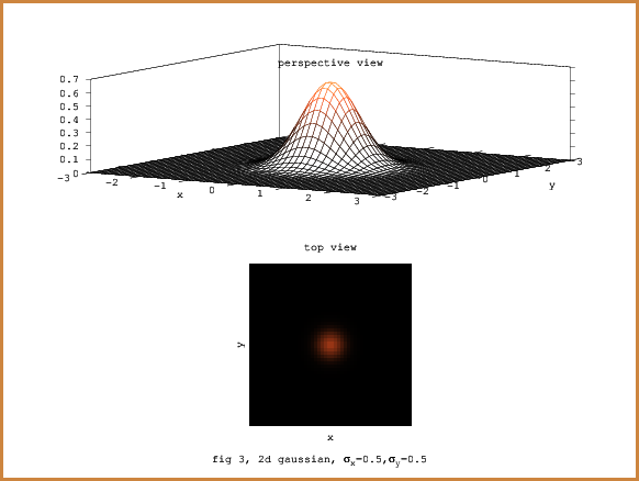
In fig-3, we have plotted the function $h(x,y) = \frac{1}{2\pi\sigma_{x}\sigma_{y}} e ^{-\frac{1}{2}(\frac{x^2}{\sigma_{x}^{2}} + \frac{y^2}{\sigma_{y}^{2}})}$ and

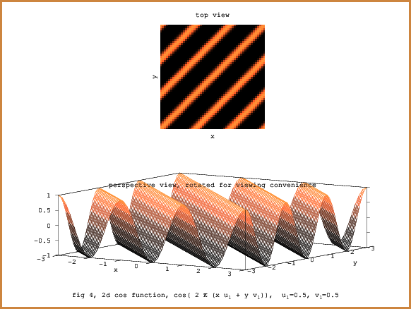
A general 2D cosine function is given by $c(x,y) = cos(2\pi (u_1 x + v_1 y))$, where $u_1, v_1$ are fixed spatial frequencies. This is shown in fig-4.

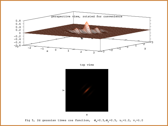
Just as in the case of the 1D gabor filter kernel, we define the 2D gabor filter kernel by the following equations. The complex 2D gabor filter kernel is given by $g(x, y)$.

$$\begin{eqnarray} \label{eqs2} g_e(x, y) & = & \frac{1}{2\pi\sigma_{x}\sigma_{y}} e ^{-\frac{1}{2}(\frac{x^2}{\sigma_{x}^{2}} + \frac{y^2}{\sigma_{y}^{2}})} cos(2\pi(u_1 x + v_1 y))\\ g_o(x, y) & = & \frac{1}{2\pi\sigma_{x}\sigma_{y}} e ^{-\frac{1}{2}(\frac{x^2}{\sigma_{x}^{2}} + \frac{y^2}{\sigma_{y}^{2}})} sin(2\pi(u_1 x + v_1 y))\\ g(x, y) & = & g_e(x, y) + i g_o(x, y) \\ & = & \frac{1}{2\pi\sigma_{x}\sigma_{y}} e ^{-\frac{1}{2}(\frac{x^2}{\sigma_{x}^{2}} + \frac{y^2}{\sigma_{y}^{2}})} e^{i2\pi(u_1 x + v_1 y)} \end{eqnarray}$$

In fig-5, we have plotted the function $g_e(x,y) = h(x, y). c(x, y)$.

Note that in fig-3, fig-4 and fig-5, the 3d perspective views are slightly rotated to accentuate their features for viewing decipherability.

Here is the octave code used for generating fig-5.

% octave code for showing  g_e(x, y) = gaussian times cosine function
%author kgeorge

clear all;
clc;
close all;
pkg load image



sigma_x = 0.5;
sigma_y = 0.5;

freq = 1.0;

%kernel size = 7 x 7
N=7;
NBY2 = floor(N/2);
tx=ty=linspace(-NBY2, NBY2, 50);
[xx, yy] = meshgrid(tx, ty);


%plot of a simple 2D gaussian
I = exp(-0.5 * ( (xx ./ sigma_x) .^2 +  (yy ./ sigma_y) .^2  ) );
I =  I .* (1.0/(2.0 * pi * sigma_x * sigma_y));


%plot of a 2D cosine wave
J = cos((xx + yy) .* (2 * pi * freq) );

colormap(copper)
s1 = subplot(2,1,2);
imshow(I .* J)
xlabel('x');
ylabel('y');

title(s1, sprintf("top view"));


colormap(copper)
s2 = subplot(2,1,1);
mesh(xx, yy, I .* J);
grid off;
view(33, 24);
xlabel('x');
ylabel('y');

title(s2, sprintf("perspective view, rotated for convenience"));



ha = axes('Position',[0 0 1 1],'Xlim',[0 1],'Ylim',[0 1],'Box','off','Visible','off','Units','normalized', 'clipping' , 'off');
text(0.5, 0.05, sprintf("fig 5, 2d gaussian times cos function,  \\sigma_x=%.1f,\\sigma_y=%.1f, u_1=%.1f, v_1=%.1f", sigma_x, sigma_y, freq, freq),'HorizontalAlignment','center','VerticalAlignment', 'top');
%save using a uility function
%saveInGithubBlog("gabor_2D_gssn_times_cos");

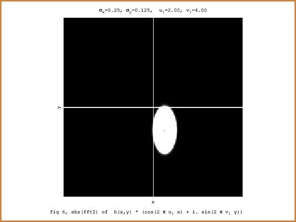
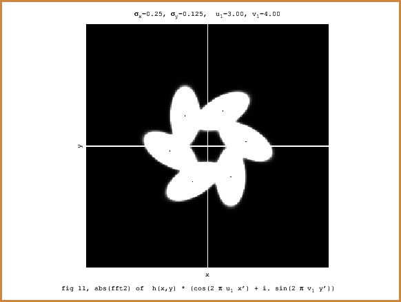
Please see \eqref{eqs3} for a derivation of the fourier transform of a gabor function as stated in \eqref{eqs2}. Shown below the image of the absolute value of the fourier transform for a gabor 2D function with $\sigma_x = 0.25, \sigma_y =0.125, u_1 = 2$ and $v_1 = 4$. Note that it is an axially aligned elliptical gaussian whose origin is shifted to $(u_1, v_1) =(2, 4)$. Please disregard the axis lines drawn. If you look carefully, in the picture there is a black dot appearing exactly at the centre of the guassian. The black dot represents the frequency $(2, 4)$ and was purposefully added to the image of the fft, just to verify the correctness of the shift.

We have now the equations for the most basic 2D gabor filter function \eqref{eqs2} and its fourier transform \eqref{eqs4}. But for using this filter function practically, we need to exploit the various ways by which this filter function can be parameterized.

First we will re-formulate \eqref{eqs2} using a more intuitive set of parameters.

A better way of expressing the parameters $\sigma_x, \sigma_y$ would be to capture the ratio between the two parameters. Thus by setting $\sigma = \sigma_y$ and $\lambda = \frac{\sigma_x}{\sigma_y}$, \eqref{eqs2} will become

$$\begin{eqnarray} \label{eqs11} g(x, y) & = & \frac{1}{2\pi\sigma_{x}\sigma_{y}} e ^{-\frac{1}{2}(\frac{x^2}{\sigma_{x}^{2}} + \frac{y^2}{\sigma_{y}^{2}})} e^{i2\pi(u_1 x + v_1 y)} \\ & = & \frac{1}{2\pi\lambda\sigma^2} \text{exp}(-\frac{((\frac{x}{\lambda})^2 + y^2)}{2\sigma^{2}}) \space \text{exp}(i2\pi(u_1 x + v_1 y)) \\ \end{eqnarray}$$

Also, consider the term $(u_1 x + v_1 y)$. If we set $f_1 = \sqrt{u_1^2 + v_1^2}$, then we can introduce an angle parameter $\theta$ where, $u_1 = f_1 cos(\theta)$ and $v_1 = f_1 sin(\theta)$. With this the equation, \eqref{eqs11} becomes,

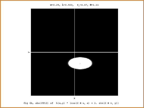
$\begin{eqnarray} \label{eqs12} g(x, y) & = \frac{1}{2\pi\lambda\sigma^2} \text{exp}(-\frac{((\frac{x}{\lambda})^2 + y^2)}{2\sigma^{2}}) \space \text{exp}(i2\pi f_1 (x cos(\theta) + y sin(\theta))) \\ \end{eqnarray}$ The fourier transform of the above representation in \eqref{eqs12} is given by \eqref{eqs13a}, which is reproduced here.

$$\begin{eqnarray} \label{eqs16} G(u, v) & = & H(u - f_1 cos(\theta) ; \lambda\sigma) H(v - f_1 sin(\theta) ; \sigma) \end{eqnarray}$$

A pictorial description of the fourier transform in \eqref{eqs16} is given by fig 6-b, which is expectedly a gaussian shifted by $(f_1 cos(\theta), f_1 sin(\theta) )$. Note the black dot, which is deliberately added at $(f_1 cos(\theta), f_1 sin(\theta) )$, to verify the correctness of the shift. Also please note that, since $lambda =0.5$, the transform is elliptical.

In fact if we plot the graph in the spatial domain, that also will be elliptical, as noted in the following figure, 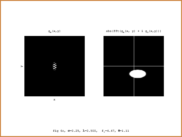. You may wonder why, the eccentricity of the elliptical figure is reversed in the transform image when compared to the spatial image, this is because, the fourier transform of a gaussian function with a given $\sigma = \sigma_1$, is a differently scaled gaussian function with whose $\sigma$ value is $\frac{1}{\sigma_1}$.

A bank of 2D gabor filter functions

Where are we heading? We need to come up with a bank of gabor filter functions, so that, effectively they cover, the entire transform space. This is shown as a rough outline in fig 6d below.

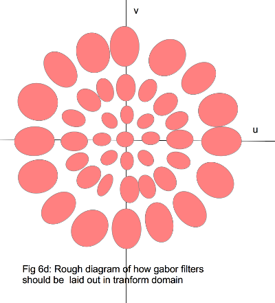
In order to achieve this varied set of gabor functions, we need to start playing around with these existing set of parameters $\sigma, \lambda, f_1, \theta$ and see how the gabor function changes. Later we will add a few more parameters.

Since we are just studying the effects of these parameters, let us continue to focus on the real part $g_e(x,y)$ of this filter.

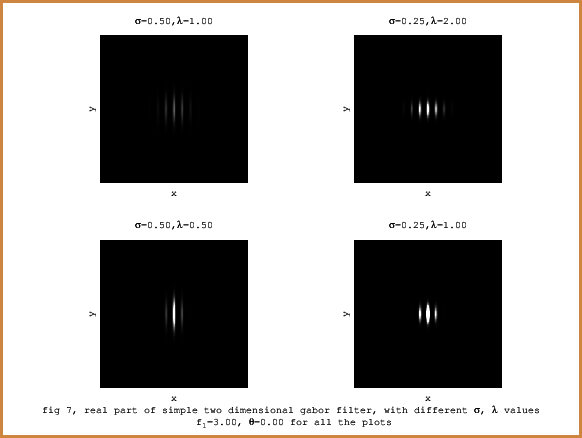In fig-7, we have plotted the real part of the gabor 2D filter with varying values of $\sigma$ and $\lambda$. Note that, as the $\lambda$-values vary, the eccentricities of the gaussian ellipse, changes, but nevertheless remains axially aligned. Also, we have kept $f_1 = 3$ and $\theta = 0$ the same.

Let us now try varying $f_1$ and $\theta$. To illustrate this, just for the purpose of clarity, we are going to plot only the cosine function, ie $cos(2\pi f_1 (x cos(\theta) + y sin(\theta)))$. Its effect on the modulation with gaussian function is self explanatory.

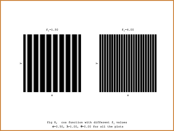
You can see from fig-8, the changes in the frequency $f_1$, of the cosine wave.

Let us vary $\theta$ now.

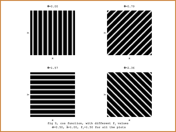
In all the considerations till now, the gaussian function was elliptical, but axially aligned. Intuitively, it would help to design better filter banks, if the gaussian function is tilted in the same manner as $\theta$. This can be accomplished by introducting a rotation transformation while computing the gaussian function.

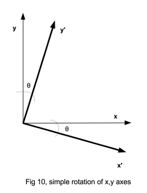
The above rotation can be accomplished by the following co-ordinate transform,

$$\begin{eqnarray} \label{eqt} R & = & \begin{bmatrix} cos(\theta) & sin(\theta) \\ -sin(\theta) & cos(\theta)\\ \end{bmatrix}\\ \begin{bmatrix} x' \\ y' \\ \end{bmatrix} & = & R \begin{bmatrix} x \\ y \\ \end{bmatrix} \end{eqnarray}$$

Shown in figure 12, above is the real part of the 2D gabor function with the effect of the gaussian function rotated by the above transformation given in \eqref{eqt}.

Another parameter that we can introduce is a phase factor $\phi$ in the sinusoidal component, which becomes, $\text{exp}(i2\pi f_1 (x cos(\theta) + y sin(\theta) + \phi))$. The cosine part of this sinusoidal function (ie the real part) is plotted below as fig 12.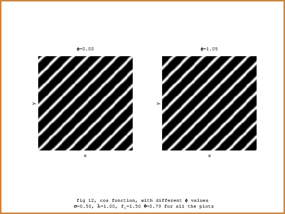

Putting all these together, the gabor kernel is defined as

$$\begin{eqnarray} \label{eqw} x' & = & x cos(\theta) + y sin(\theta) \\ y' & = & -x sin(\theta) + y cos(\theta) \\ g(x, y) & = & \frac{1}{2\pi\lambda\sigma^2} \text{exp}(-\frac{((\frac{x'}{\lambda})^2 + y'^2)}{2\sigma^{2}}) \space \text{exp}(i2\pi f_1 (x' + \phi )) \\ \end{eqnarray}$$

\eqref{eqs22} gives the fourier transform of such a gabor function described in \eqref{eqw}. Shown below is the absolute value of the fourier transform of such an example gabor function, with $\sigma_x = 0.25, \sigma_y =0.125, u_1 =2, u_2 =4$ and $\alpha = \frac{\pi}{2}$. Note that the spectrum is still an axially aligned ellipse and is shifted to $u_1 = 2, v_1 = 4$. Please disregard the axis lines drawn. Also, we have added a black dot to the transform image at the frequency $(2, 4)$, to signify and verify the correctness of the shift.

Appendix

Derivation of fourier transform of a 1-D gaussian function.

How do we find the fourier transform $\mathscr{F}(h(t)) = H(f)$ of a one dimensional gaussian function $h(t)$?

For a general function $p(t)$, the fourier transform $\mathscr{F}(p(t)) = P(f)$ is given by \eqref{eqv}.

On a simpler note, let us work on a simple function $h(t) = e^{-at^2}$ and try to find its fourier transform $H(f)$.

$$\begin{eqnarray} \label{eqc} H(f) & = & \int_{-\infty}^{\infty} h(t) e^{-i2\pi f t} dt \\ & = & \int_{-\infty}^{\infty} e^{-at^2} e^{-i2\pi f t} dt \\ & = & \int_{-\infty}^{\infty} e^{-at^2} (cos(2\pi f t) - i. sin(2\pi f t)) dt \\ & = & \int_{-\infty}^{\infty} e^{-at^2} cos(2\pi f t) - i. \int_{-\infty}^{\infty} e^{-at^2} sin(2\pi f t) dt \end{eqnarray}$$

Please remember that for an odd function $o(t)$, $\int_{-\infty}^{0} o(t) = -\int_{0}^{\infty} o(t)$ and so $\int_{-\infty}^{\infty} o(t) = 0$.

Since $e^{-at^2}$ is an even function and $sin(2\pi f t)$ is an odd function, $\int_{-\infty}^{\infty} e^{-at^2} sin(2\pi f t) = 0$.

So the above equation simplifies to

$$\begin{eqnarray} \label{eqd} H(f) & = & \int_{-\infty}^{\infty} e^{-at^2} cos(2\pi f t) \space dt\\ & = & 2 \int_{0}^{\infty} e^{-at^2} cos(2\pi f t) \space dt \end{eqnarray}$$

Using [1], Abramovitz et. al., $\int_{0}^{\infty} e^{-at^2} cos(2xt) \space dt = \frac{1}{2}\sqrt{\frac{\pi}{a}} e^{-\frac{x^2}{a}}$. So the above equation translates to,

$$\begin{eqnarray} \label{eqe} H(f) & = & \sqrt{\frac{\pi}{a}} e^{-\frac{\pi^2 f^2}{a}} \end{eqnarray}$$

Putting $a = \frac{1}{2\sigma^2}$, in \eqref{eqe}, fourier transform $H(w)$ of $h(t)$ in \eqref{eqa} is,

$$\begin{eqnarray} \label{eqf} H(f) & = & \frac{1}{\sqrt{2\pi}\sigma} \sqrt{2\pi}\sigma e^{-2\pi^2 f^2\sigma^2} \\ & = & e^{-2\pi^2 f^2\sigma^2} \\ \end{eqnarray}$$

Derivation of fourier transform of a 2D gaussian function.

A 2D gaussian function is given by \eqref{eqaa} $\begin{eqnarray} \label{eqaa} h(x,y) & = & \frac{1}{2\pi\sigma_{x}\sigma_{y}} e ^{-\frac{1}{2}(\frac{x^2}{\sigma_{x}^{2}} + \frac{y^2}{\sigma_{y}^{2}})} \end{eqnarray}$

Note that \eqref{eqaa} can be written as, $\begin{eqnarray} \label{eqab} h_1(x) & = & \frac{1}{\sqrt{2\pi}\sigma_{x}} e ^{ - 0.5 \frac{x^2}{\sigma_{x}^{2}}} \\ h_2(y) & = & \frac{1}{\sqrt{2\pi}\sigma_{y}} e ^{ - 0.5 \frac{y^2}{\sigma_{y}^{2}}} \\ h(x, y) & = & h_1(x) h_2(y) \end{eqnarray}$

Given any 2D function $p(x,y)$, its fourier transform $\mathscr{F}(p(x, y) = P(u,v)$ is given by

$$\begin{eqnarray} \label{eqac} P(u, v) & = & \int_{-\infty}^{\infty} \int_{-\infty}^{\infty} p(x, y) e^{-i2\pi(ux + vy)} \space dx dy \end{eqnarray}$$

A 2D function $p(x, y)$ is separable, if it can be written as $p(x,y) = p_{1}(x).p_{2}(y)$. If $P_{1}(u)$ and $P_{2}(v)$ are the fourier transforms of $p_{1}$ and $p_{2}$ respectively, then,

$$\begin{eqnarray} \label{eqad} P(u, v) & = & \int_{-\infty}^{\infty} \int_{-\infty}^{\infty} p_1(x) p_2(y) e^{-i2\pi(ux + vy)} \space dx dy \\ & = & \int_{-\infty}^{\infty} \int_{-\infty}^{\infty} p_1(x) e^{-i2\pi ux} dx \space p_2(y) e^{-i2\pi vy} dy \\ & = & P_1(u) P_2(v) \end{eqnarray}$$

From \eqref{eqab}, \eqref{eqad}, and \eqref{eqf}, we derive the fourier transform $\mathscr{F}(h(x, y)) = H(u, v)$ of a gaussian as,

$$\begin{eqnarray} \label{eqaf} H(u, v) & = & e^{-2\pi^2(u^2\sigma_{x}^2 + v^2\sigma_{y}^2 )} \end{eqnarray}$$

Derivation of fourier transform of sine and cosine functions

Consider a simple cosine and a sine function, $c(t)$ and $s(t)$ respectively, what would be their fourier transforms $\mathscr{F}(c(t)) = C(f)$ and $\mathscr{F}(s(t)) = S(f)$?

$$\begin{eqnarray} \label{eqh} c(t) & = & cos(2\pi f_1 t) \\ & = & \frac{1}{2} ( \text{exp}(-i2\pi f_1 t) + \text{exp}(i2\pi f_1 t) ) \end{eqnarray}$$ $$\begin{eqnarray} \label{eqg} s(t) & = & sin(2\pi f_1 t) \\ & = & \frac{i}{2} ( e^{-i2\pi f_1 t} - e^{i2\pi f_1 t} ) \end{eqnarray}$$

From \eqref{eqh},

$$\begin{eqnarray} \label{eqi} C(f) & = & \int_{-\infty}^{\infty} c(t) e^{-i2\pi f t} dt \\ & = & \int_{-\infty}^{\infty} \frac{1}{2} ( e^{-i2\pi f_1 t} + e^{i2\pi f_1 t} ) e^{-i2\pi f t} dt \\ & = & \int_{-\infty}^{\infty} \frac{1}{2} ( e^{-i2\pi(f + f_1) t} + e^{-i2\pi (f - f_1) t} ) dt \\ \end{eqnarray}$$

Consider the integral $\int_{-\infty}^{\infty} e^{-i2\pi f t} dt$, That is the fourier transform $I(f)$ of the identity function $i(t)=1$.

The fourier inversion theorem states the following, if $P(f) = \int_{-\infty}^{\infty} e^{-i2\pi f t} p(t) \space dt$, then $\int_{-\infty}^{\infty} e^{i2\pi f x} P(f) df = p(x)$. For a proof, please see [2], Proof of Fourier inversion theorem

Now considering, the dirac delta function $\delta(t)$ with the property $\int_{-\infty}^{\infty} \delta(t-a) p(t) = p(a)$, the integral below, evaluates to $1$ or the identity function $i(x)$.

$$\begin{eqnarray} \label{eqj} \int_{-\infty}^{\infty} e^{i2\pi f x} \delta(f) df & = & 1 \\ & = & i(x) \end{eqnarray}$$

Applying the fourier inversion theorem, \eqref{eqj} translates to

$$\begin{eqnarray} \label{eqk} \int_{-\infty}^{\infty} e^{-i2\pi f x} i(x) dx & = & \delta(f) \end{eqnarray}$$

So \eqref{eqi} can be continued as,

$$\begin{eqnarray} \label{eql} C(f) & = & \int_{-\infty}^{\infty} \frac{1}{2} ( e^{-i2\pi(f + f_1) t} + e^{-i2\pi (f - f_1) t} ) dt \\ & = & \frac{1}{2} (\delta(f + f_1) + \delta(f - f_1)) \\ \end{eqnarray}$$

Similarly, from \eqref{eqg}, fourier transform $S(f)$of sine function $s(t) = sin(2\pi f_1 t)$ is given by,

$$\begin{eqnarray} \label{eqm} S(f) & = & \frac{i}{2} (\delta(f + f_1) - \delta(f - f_1)) \end{eqnarray}$$

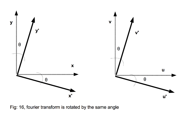
Fourier transform of a rotated 2D signal

Let $\mathscr{F}(p(x, y)) = P(u, v)$. Consider the rotation given in \eqref{eqt}, and shown in fig 10.

$$\begin{eqnarray} \label{eqm2} R & = & \begin{bmatrix} cos(\theta) & sin(\theta) \\ -sin(\theta) & cos(\theta)\\ \end{bmatrix}\\ \begin{bmatrix} x' \\ y' \\ \end{bmatrix} & = & R \begin{bmatrix} x \\ y \\ \end{bmatrix}\\ \end{eqnarray}$$

Another way to express this relationship is $x'$ ad $y'$ are functions of $x, y$ given by,

$$\begin{eqnarray} \label{eqm2a} x'(x, y) & = & x cos(\theta) + y sin(\theta) \\ y'(x, y) & = & -x sin(\theta) + y cos(\theta) \end{eqnarray}$$

Similarly, $x$ ad $y$ are functions of $x', y'$ given by, $\begin{eqnarray} \label{eqm3} x(x', y') & = & x' cos(\theta) - y' sin(\theta) \\ y(x', y') & = & x' sin(\theta) + y' cos(\theta) \end{eqnarray}$

Please note the following identity for taking derivatives for transformations,

$\begin{eqnarray} \label{eqm4} dx dy & = & \begin{vmatrix} \frac{\partial x}{\partial x' } & \frac{\partial x}{ \partial y'}\\ \frac{\partial y}{\partial x'} & \frac{\partial y}{\partial y'} \\ \end{vmatrix} dx' dy' \\ & = & \begin{vmatrix} cos(\theta) & -sin(\theta)\\ sin(\theta) & cos(\theta) \\ \end{vmatrix} dx' dy' \\ & = & dx' dy' \\ \end{eqnarray}$ If we set, $\begin{eqnarray} \label{eqm5} u' & = & u cos(\theta) + y sin(\theta) \\ v' & = & -u sin(\theta) + y cos(\theta) \end{eqnarray}$

By \eqref{eqac}, \eqref{eqm4} and \eqref{eqm5}, and if we denote $q(x, y) = p(x'(x, y), y'(x, y))$, the the corresponding fourier transform $\mathscr{F}(q(x,y)) = Q(u, v)$ is given by,

$$\begin{eqnarray} \label{eqac2} Q(u, v) & = & \int_{-\infty}^{\infty} \int_{-\infty}^{\infty} p(x', y') \space \text{exp}(-i2\pi(ux + vy)) \space dx dy \\ & = & \int_{-\infty}^{\infty} \int_{-\infty}^{\infty} p(x', y') \space \text{exp}(-i2\pi(ux' cos(\theta) - uy' sin(\theta) + vx' sin(\theta) + vy' cos(\theta))) \space dx dy \\ & = & \int_{-\infty}^{\infty} \int_{-\infty}^{\infty} p(x', y') \space \text{exp}(-i2\pi(ux' cos(\theta) + vx' sin(\theta) - uy' sin(\theta) + vy' cos(\theta))) \space dx dy \\ & = & \int_{-\infty}^{\infty} \int_{-\infty}^{\infty} p(x', y') \space \text{exp}(-i2\pi(u'x' + v'y') \space dx dy \\ & = & \int_{-\infty}^{\infty} \int_{-\infty}^{\infty} p(x', y') \space \text{exp}(-i2\pi(u'x' + v'y') \space dx' dy' \\ & = & P(u',v') \end{eqnarray}$$

This means that, fourier transform $Q(u,v)$ of a rotated signal $q(x,y) = p(x'(x,y), y'(x, y))$, is the fourier transform $P(u'(u,v), v'(u,v))$ which will be the fourier transform $P(u,v)$ after a rotation of $\theta$, as shown in the figure below.

Derivation of fourier transform of a 2D gabor function.

Since there are several variants of the 2D functions mentioned in this article, let us first focus on the most basic of these, as described in \eqref{eqs2}.

fourier transform of simple 2D gabor function given in \eqref{eqs2}

From \eqref{eqs2},

$$\begin{eqnarray} \label{eqs3} g(x, y) & = & g_e(x, y) + i g_o(x, y) \\ & = & \frac{1}{2\pi\sigma_{x}\sigma_{y}} \space \text{exp}(-\frac{1}{2}(\frac{x^2}{\sigma_{x}^{2}} + \frac{y^2}{\sigma_{y}^{2}})) \space \text{exp}(i2\pi(u_1 x + v_1 y)) \\ \text{Let} \space g_1(x) & = & \frac{1}{\sqrt{2\pi}\sigma_{x}} \space \text{exp} (- \frac{x^2}{2\sigma_{x}^{2}}) \space \text{exp}(i2\pi u_1 x) \\ \text{and} \space g_2(y) & = & \frac{1}{\sqrt{2\pi}\sigma_{y}} \space \text{exp} (- \frac{y^2}{2\sigma_{y}^{2}}) \space \text{exp}(i2\pi v_1 y) \\ \text{then}, \space g(x, y) & = & g_1(x) \space g_2(y) \end{eqnarray}$$

So by the separability feature of fourier transform as shown in \eqref{eqad} and by \eqref{eqp2}, the fourier transform $\mathscr{F}(g(x,y)) = G(u, v)$ of a 2D gabor function given in \eqref{eqs3} is,

$$\begin{eqnarray} \label{eqs4} G(u, v) & = & G_1(u) \space G_2(v) \\ & = & H(u - u_1) H(v - v_1) \\ \end{eqnarray}$$

Note that $H(u - u_1)$ is $\mathscr{F}(h(t))$ of the gaussian $h(t)$, translated to the frequency $u_1$.

Now let us move to more general and parametric forms of the 2D gabor function.

fourier transform of 2D gabor function (with $\lambda$ and $\theta$ parameters) as described in \eqref{eqs12}

We will be working with \eqref{eqs12}.

The fourier transform of the 1D gaussian function $\mathscr{F}(h(t)) = H(f)$, can be expressed moe accurately with the parameter $\sigma$ as $H(f; \sigma)$.

So we can rewrite \eqref{eqf} as

$$\begin{eqnarray} \label{eqs14} H(f ; \sigma) & = & \text{exp}(-2\pi^2 f^2\sigma^2) \\ \end{eqnarray}$$

From \eqref{eqs12} $\begin{eqnarray} \label{eqs13} g(x, y) & = & \frac{1}{2\pi\lambda\sigma^2} \text{exp}(-\frac{((\frac{x}{\lambda})^2 + y^2)}{2\sigma^{2}}) \space \text{exp}(i2\pi f_1 (x cos(\theta) + y sin(\theta))) \\ \text{Let} \space g_1(x) & = & \frac{1}{\sqrt{2\pi}\lambda\sigma} \text{exp}(- \frac{x^2}{2(\lambda \sigma)^{2}}) \space \text{exp}(i2\pi f_1 x cos(\theta) ) \\ \text{and} \space g_2(y) & = & \frac{1}{\sqrt{2\pi}\sigma} \text{exp}(- \frac{y^2}{2\sigma^{2}}) \space \text{exp}(i2\pi f_1 y sin(\theta) ) \\ g(x, y) & = & g_1(x) \space g_2(y) \end{eqnarray}$

So again by the separability feature of fourier transform as shown in \eqref{eqad} and by \eqref{eqp2} , $\mathscr{F}(g(x,y))$will translate to

$$\begin{eqnarray} \label{eqs13a} G(u, v) = H(u - f_1 cos(\theta); \lambda \sigma ) \space H(v - f_1 sin(\theta); \sigma) \end{eqnarray}$$

fourier transform of 2D gabor function (with $\lambda$, $\theta$ and rotated gaussian)

The most generalized form of the 2D gabor function was given by \eqref{eqw}, which is reproduced below,

$$\begin{eqnarray*} g(x, y) & = & \frac{1}{2\pi\lambda\sigma^2} \text{exp}(-\frac{((\frac{x'}{\lambda})^2 + y'^2)}{2\sigma^{2}}) \space \text{exp}(i2\pi f_1 (x' + \phi )) \\ \end{eqnarray*}$$

Let us try to come up with a formula for its fourier transform $\mathscr{F}(g(x,y) = G(u, v)$.

Consider the function, $p(x, y) = \frac{1}{2\pi\lambda\sigma^2} \text{exp}(-\frac{((\frac{x}{\lambda})^2 + y^2)}{2\sigma^{2}}) \space \text{exp}(i2\pi f_1 (x + \phi ))$ in \eqref{eqs17},

$\begin{eqnarray} \label{eqs17} p(x, y) & = & \frac{1}{2\pi\lambda\sigma^2} \text{exp}(-\frac{((\frac{x}{\lambda})^2 + y^2)}{2\sigma^{2}}) \space \text{exp}(i2\pi f_1 (x + \phi ))\\ p_1(x) & = & \frac{1}{\sqrt{2\pi}\lambda\sigma} \text{exp}(- \frac{x^2}{2(\lambda \sigma)^{2}}) \space \text{exp}(i2\pi f_1 x ) \\ p_2(y) & = & \frac{1}{\sqrt{2\pi}\sigma} \text{exp}(- \frac{y^2}{2\sigma^{2}})\\ p(x, y) & = & p_1(x) \space p_2(y) \space \text{exp}(i 2 \pi f_1 \phi) \end{eqnarray}$ Note that $g(x, y) = p(x'(x,y), y'(x,y))$. Here we used the notation in \eqref{eqm2a} that $x'$, and $y'$ are functions of $x$ and $y$.

The fourier transform $\mathscr{F}(p(x,y) = P(u,v)$ derived below.

Due to the separability feature of the fourier transform, we have,

$$\begin{eqnarray} \label{eqs5} P(u, v) = H(u - f_1; \lambda \sigma) \space H(v; \sigma) \space \text{exp}(i 2 \pi f_1 \phi) \end{eqnarray}$$ $$\begin{eqnarray} \label{eqs18} G(u, v) & = & \mathscr{F} (g(x, y)) \\ & = & \mathscr{F} (p(x'(x,y), y'(x,y)))\\ & = & P(u', v') \space \text{as in} \space \eqref{eqac2} \space \text{where} \\ u' & = & u cos(\theta) + v sin(\theta)\\ v' & = & -u sin(\theta) + v cos(\theta)\\ \end{eqnarray}$$

Finally we have,

$$\begin{eqnarray} \label{eqs22} G(u, v) & = & H(u' - f_1; \lambda \sigma) \space H(v'; \sigma) \space \text{exp}(i 2 \pi f_1 \phi) \end{eqnarray}$$

References

1. Abramowitz, M. and Stegun, I. A. (Eds.). Handbook of Mathematical Functions with Formulas, Graphs, and Mathematical Tables, 9th printing. New York: Dover, p. 302,

2. [Proof of Fourier inversion theorem] (http://math.columbia.edu/~nsnyder/tutorial/lecture3.pdf)

---

---

blog comments powered by Disqus

Published

Tags

• image processing 1
• fourier transform 1
• convolution 1
• signal processing 1
• feature extraction 1