HOG implementation and object detection
Histogram Oriented Gradient (HOG) has been proven to be a versatile strategy in detecting objects in cluttered environments. Since the concept is simple enough, we came up with a c++ implementation which was used for detecting passing cars on two lane high ways.
 Also, please see this video
Implementation details
environment
We used C++ for writing low level routines starting from the block level. (ie every thing that deal with blocks, cells, pixels are in C++). We used boost-python binding mechanism to bind the C++ to python. The version of boost used was 1.55.0.
interfacing with image data
On the python side, since we used cv2 module, the image comes as a numpy array. We use the code given by NumPyArrayData to access the internals of the numpy array, from the c++ side.
- Example c++ code
#include <boost/python.hpp>
#include <boost/numpy.hpp>
#include "NumPyArrayData.hpp"

namespace bp = boost::python;
namespace np = boost::numpy;

//example code to get the (r,c) th pixel, r==rowIndex, c==columnIndex
unsigned char getPixel( np::ndarray& img, int r, int c) {
    NumPyArrayData< unsigned char > arr_data(arr);
    return arr_data(r, c);
}

//example code to set the (r,c) th pixel, r==rowIndex, c==columnIndex
void setPixel( np::ndarray& img, int i, int j, unsigned char pixelValue) {
    NumPyArrayData< unsigned char > arr_data(arr);
    arr_data(r, c) = pixelValue;
    return;
}


// Expose the above methods to Python
BOOST_PYTHON_MODULE(hogModule) {
    np::initialize();
    bp::def("getPixel", &getPixel);
    bp::def("setPixel", &setPixel);
}
Compile the above code into a binary hogModule.so and place it accessible to python. Alternatively, put the .so
in a convenient directory Eg: ./myBins/hogModule.so and invoke python with the following environment PYTHONPATH=./myBins/:$PYTHONPATH python
import numpy as np
import cv2, cv
import hogc

def manipulateImage(grayScaleImagePathName):
    img = cv2.imread(grayScaleImagePathName)
    print "The (r=0,c=0)th pixel of %s is: %d" %
        (imagePathName, hogModule.getPixel(img, 0, 0))
    imagePathName, hogModule.setPixel(img, 0, 0, ) = 128
    print "The (r=0,c=0)th pixel of %s is: %d, it should be 128" %
        (imagePathName, hogModule.getPixel(img, 0, 0))


if __name__ == "__main__":
    manipulateImage("./data/myGrayScale.png")
HOG parameters
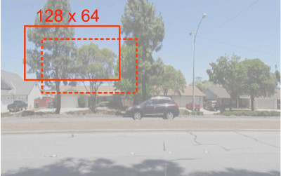
sliding window
The input video was scaled down to 640 x 360 pixels by cv2.pyrDown. We used a sliding window of size 128 x 64 pixels over each frame of the video.
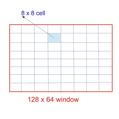
cells
Each sliding window (128 pixels x 64 pixels) was divided into (8 pixel x 8 pixel) cells. So there would be (16 x 8) cells.
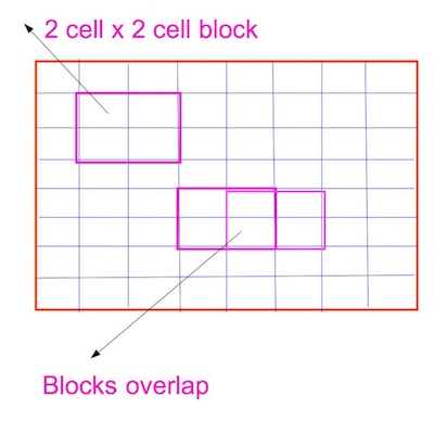
blocks
A 2 cell x 2 cell combination would form a block. Because the blocks overlap 50% on the rows and columns, there would be 15 x 7 = 105 such blocks in a sliding window.
pre-processing a sliding window
For each sliding window, do the following transformations.
- gamma-correction
We pre-processed each sliding window of RGB pixels (not gray scale) to gamma-correction. Since all our images are from a single camera, may be there was no need for this. Based on the following c++ code, the gamma correction
was invoked in python as hogModule.gammaCorrect(numpyImg, 2.2, True)
#include <boost/python.hpp>
#include <boost/python/suite/indexing/vector_indexing_suite.hpp>
#include <boost/numpy.hpp>
#include <math.h>

#include "NumPyArrayData.hpp"

namespace bp = boost::python;
namespace np = boost::numpy;


void gammaCorrect( np::ndarray& imgArr, float gamma, bool reverse ) {
    NumPyArrayData<unsigned char> imgData(imgArr);
    Py_intptr_t const *pShape =   imgArr.get_shape();
    //we need color now
    assert( imgArr.get_nd() == 3);

    int h = *(pShape+0);
    int w = *(pShape+1);
    int d = *(pShape+2);
    float lut[256];
    float reciprocal255 = 1.0f/255.0f;
    float gammaExponent =  (reverse) ? (1.0f/gamma) : gamma;
    for(int i=0; i < 256; ++ i) {
        lut[i] = pow(i * reciprocal255, gammaExponent);
    }

    for(int i=0; i < h; ++i) {
        for(int j=0; j < w; ++j) {
            imgData(i,j,0) = round(lut[imgData(i,j,0)] * 255);
            imgData(i,j,1) = round(lut[imgData(i,j,1)] * 255);
            imgData(i,j,2) = round(lut[imgData(i,j,2)] * 255);
        }
    }
}
// Expose classes and methods to Python
BOOST_PYTHON_MODULE(hogModule) {
    np::initialize();
    bp::def("gammaCorrect", &gammaCorrect,  bp::args("imgArr", "gamma", "reverse"));
}
HOG descriptor calculation
For each sliding window, for each block (there are 15 x 7 such blocks), for each cell (there are 2 x 2 cells), calculate the gradients of each inner pixel and bin this gradient to a 9 bin histogram. The gradients for each cell is calculated as follows.
namespace Kg {

    template<typename T>
    struct Point2 {
        T r;
        T c;
        Point2():r(0),c(0){}
        Point2(T r, T c):r(r),c(c){}
        T get_r()const { return r;}
        T get_c()const {return c;}
        void set_r(T r_){ r = r_;}
        void set_c(T c_){ c = c_;}
    };

    typedef Point2<int> Point2i;
    typedef Point2<float> Point2f;


    template<typename K>
    struct EpsilonEq {
        static const K epsilon_;
        bool operator()(const K &l, const K &r) {
            return abs(l-r) < epsilon_;
        }
    };


    template<>
    struct EpsilonEq<float> {
        typedef float K;
        static constexpr float epsilon_ =  0.000001f;
        bool operator()(const K &l, const K &r) {
            return abs(l-r) < epsilon_;
        }
    };
}

void computeAngleAndMagnitudeUnSigned( const Kg::Point2f & inputPixelDiff, float &angle, float &magnitude) {
    angle = atan(inputPixelDiff.r/inputPixelDiff.c);

    if(inputPixelDiff.r == 0) {
        angle = 0.0f;
    }
    angle = angle + M_PI/2.0;
    Kg::EpsilonEq<float> isEpsilonEqual;
    if(!(((angle > 0) || isEpsilonEqual(angle, 0)) && ((angle < M_PI) || isEpsilonEqual(angle, M_PI)))) {
        assert(false);
    }
    am.set_a(angle);
    magnitide = sqrt(inputPixelDiff.c*inputPixelDiff.c + inputPixelDiff.r * inputPixelDiff.r);
}

void computeCellGradients(
        np::ndarray& imgArr,
        int r_cell, int c_cell, std::vector<float> &angles, std::vector<float> &magnitudes) {
        angles.clear();
        magnitudes.clear();
        const int numPixelsInCellPerSide=8;
        NumPyArrayData<unsigned char> imgData(imgArr);
        for(int r = r_cell+1; r < r_cell + numPixelsInCellPerSide - 1; ++r) {
            for(int c = c_cell+1; c < c_cell + numPixelsInCellPerSide - 1; ++c ) {
                Kg::Point2f imgPixelDiff = Kg::Point2f(
                    (imgData(r+1,c) - imgData(r-1,c)) * 0.5,
                    (imgData(r,c+1) - imgData(r,c-1)) * 0.5
                );
                AngleAndMagnitude am;
                int rOffset = r - r_cell;
                int cOffset = c - c_cell;
                float angle;
                float magnitude;
                float weight = gaussianWeighter(rOffset,cOffset)

                computeAngleAndMagnitudeUnSigned(imgPixelDiff, angle, magnitude);
                angles.push_back(angle);
                magnitudes.push_back(magnitude * weight);
            }
        }
    }
Please note that in each cell, we are weighting the magnitude by a 2d gaussian (the code is not provided here). The gaussian weighting is done on a block basis.
We make a histogram of the angles (who are unsigned and varies from 0 to 180 degrees), into 9 bins. An angle is linearly split into neighboring bins, based its proximity to neighboring bin centers. We scale the fraction of the entry of angle into a bin by the corresponding fraction of its magnitude.
Eg: Suppose 1.5 and 2.5 are two neighboring bin centers, and (angle=1.8, magnitude=30.0) is a sample, the contributing factor to bin centered at 1.5 is 0.7 and the contributing factor to the bin centered at 2.5 is 0.3. So 0.7 * 30.0 is added to the bin centered at 1.5 and 0.3 * 30.0 is added to the bin centered at 2.5
The histograms of all cells are concatenated to form a block histogram. We do L2 normalization on the block histogram. There would be 4 * 9 entries for this normalized block histogram.
There are 105 blocks in a sliding window which give rise to 4 x 9 x 105 = 3780 entries for the descriptor.
classifier training.
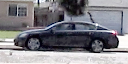
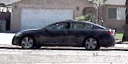
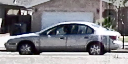
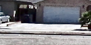
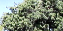
We collected good samples and bad samples of the sliding window. Some examples of good samples are.
good samples
bad samples
classification
We used the python module ‘sklearn’ to enforce the classification. Suppose ‘X’ is a n x 3780 matrix which hold all the descriptors of n sample sliding windows, and ‘y’ is the n x 1 matrix holding the correpsonding labels, the following code was used to generate the classifier.
import sklearn.svm as skl

def learn(X, y):
    clf = skl.SVC(kernel="linear", verbose=True, probability=True)
    return clf.fit(X, y)
For each of the input sample sliding window X, which is a 1 x 3780 matrix, the follwing code was used to detect whether it is a car or not
import sklearn.svm as skl

def predict(sliding_window_image):
    gammaCorrect(sliding_window_image)
    normalizedImage = normalize(sliding_window_image)
    convertedImage = cv2.cvtColor( normalizedImage, cv2.COLOR_BGR2GRAY)
    //compute hog parametsrs
    hog_descriptors = np.zeros((3780))

    //fill in the routne for computing 3780 hog descriptors
    //compute_hog(convertedImage, hog_descriptors)

    prob = clf.predict_proba(hog_descriptors)
    if (prob > 0.85):
        print "yes car"
    else:
        print "no car"
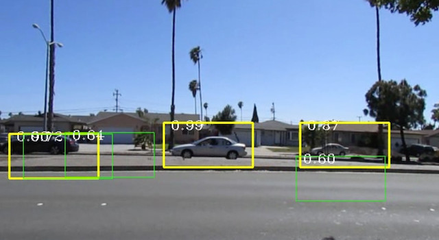
non-maxima suppression
All the “yes car” sample sliding windows for a frame would be sorted in descending order of the result probability and all the neighboring yes samples of a maxima would be suppressed. A neighborhood window of 20 pixels x 20 pixels is used.
Speed
The current implementation is not gpu accelerated and it takes 5.2 minutes for each input video frame.
Scale
The current implementation does not tolerate wide variation in scales of cars. Hence it fails to find cars which are far way and very near.
The implementation has been tailored to detect cars passing though the opposite two lanes in a 4 lane-highway (two lanes each way). Even then we have vehicles coming
in various sizes, small cars to big min vans. To accommodate a good chunk of vehicles, we used a sliding window of 150 pixels x 75 pixels in a 640 x 360 input frame,
Each sliding window would be resized to 128 x 64, by cv2.resize
blog comments powered by Disqus